PBxplore API cookbook — Visualize protein deformability
Table of Contents
Note
This page is initialy a jupyter notebook. You can see a notebook HTML render of it or download the notebook itself.
Protein Blocks are great tools to study protein deformability. Indeed, if the block assigned to a residue changes between two frames of a trajectory, it represents a local deformation of the protein rather than the displacement of the residue.
The PBxplore API allows to visualize Protein Block variability throughout a molecular dynamics simulation trajectory.
from __future__ import print_function, division
from pprint import pprint
from IPython.display import Image, display
import matplotlib.pyplot as plt
%cd ../../../
%matplotlib inline
/home/docs/checkouts/readthedocs.org/user_builds/jbarnoudpbxplore/checkouts/sphink-clean
import pbxplore as pbx
Here we will look at a molecular dynamics simulation of the barstar. As we will analyse Protein Block sequences, we first need to assign these sequences for each frame of the trajectory.
# Assign PB sequences for all frames of a trajectory
trajectory = 'demo2/barstar_md_traj.xtc'
topology = 'demo2/barstar_md_traj.gro'
sequences = []
for chain_name, chain in pbx.chains_from_trajectory(trajectory, topology):
    dihedrals = chain.get_phi_psi_angles()
    pb_seq = pbx.assign(dihedrals)
    sequences.append(pb_seq)
Block occurences per position
The basic information we need to analyse protein deformability is the
count of occurences of each PB for each position throughout the
trajectory. This occurence matrix can be calculated with the
pbxplore.analysis.count_matrix() function.
count_matrix = pbx.analysis.count_matrix(sequences)
count_matrix is a numpy array with one row per PB and one column per
position. In each cell is the number of time a position was assigned to
a PB.
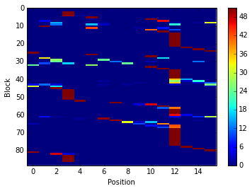
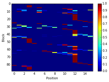
We can visualize count_matrix using Matplotlib as any 2D numpy
array.
im = plt.imshow(count_matrix, interpolation='none', aspect='auto')
plt.colorbar(im)
plt.xlabel('Position')
plt.ylabel('Block')
<matplotlib.text.Text at 0x7f4beb571210>
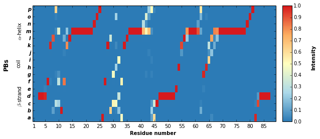
PBxplore provides the pbxplore.analysis.plot_map() function to
ease the visualization of the occurence matrix.
pbx.analysis.plot_map('map.png', count_matrix)
!rm map.png
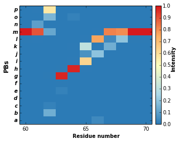
The pbxplore.analysis.plot_map() helper has a residue_min
and a residue_max optional arguments to display only part of the
matrix. These two arguments can be pass to all PBxplore functions that
produce a figure.
pbx.analysis.plot_map('map.png', count_matrix,
                      residue_min=60, residue_max=70)
!rm map.png
Note that matrix in the the figure produced by
pbxplore.analysis.plot_map() is normalized so as the sum of each
column is 1. The matrix can be normalized with the
pbxplore.analysis.compute_freq_matrix().
freq_matrix = pbx.analysis.compute_freq_matrix(count_matrix)
im = plt.imshow(freq_matrix, interpolation='none', aspect='auto')
plt.colorbar(im)
plt.xlabel('Position')
plt.ylabel('Block')
<matplotlib.text.Text at 0x7f4beb217390>
Protein Block entropy
The \(N_{eq}\) is a measure of variability based on the count matrix
calculated above. It can be computed with the
pbxplore.analysis.compute_neq() function.
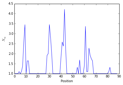
neq_by_position = pbx.analysis.compute_neq(count_matrix)
neq_by_position is a 1D numpy array with the \(N_{eq}\) for each
residue.
plt.plot(neq_by_position)
plt.xlabel('Position')
plt.ylabel('$N_{eq}$')
<matplotlib.text.Text at 0x7f4beb1c9850>
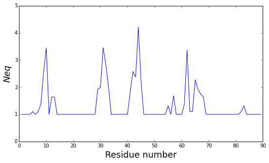
The pbxplore.analysis.plot_neq() helper ease the plotting of the
\(N_{eq}\).
pbx.analysis.plot_neq('neq.png', neq_by_position)
!rm neq.png
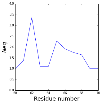
The residue_min and residue_max arguments are available.
pbx.analysis.plot_neq('neq.png', neq_by_position,
                      residue_min=60, residue_max=70)
!rm neq.png
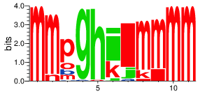
Display PB variability as a logo
pbx.analysis.generate_weblogo('logo.png', count_matrix)
display(Image('logo.png'))
!rm logo.png

pbx.analysis.generate_weblogo('logo.png', count_matrix,
                              residue_min=60, residue_max=70)
display(Image('logo.png'))
!rm logo.png